Abstract
In general you will use named ranges in Excel to avoid hard coded references to input cells or to output cells. If you assign names to important cells, the references to them will be automatically updated in case of insertions or deletions of rows or columns.
Here we like to use named ranges in Excel to efficiently implement a simple solution with nested worksheet formulas which do not need future amendments:
We want to organize a simple round tobin tournament of an (almost) arbitrary number of players, where each player will play exactly one game against each other player. For ease of reference we define that player 1 will play with White in round 1 (i.e. has a home game).
The simple nested formulas we can implement with named ranges. All necessary parameters are the column and row positions relative to the anchor point in the top left corner of the pairings table.
Please note: A named range is evaluated whenever a formula that refers to it is evaluated. This means it will be evaluated as often as it appears in different formulas which are being evaluated. Unreferenced named ranges will not be evaluated, not even by a full recalculation (CTRL + ALT + F9).
Developing a Formula Solution for a Round Robin Tournament
After defining the kind of tournament we just need one parameter for this round robin tournament: the number of players.
We like to present all games to play in a simple table. Example:
| Table 1 | Table 2 | Table 3 | |
|---|---|---|---|
| Round 1 | 1 - 6 | 5 - 2 | 3 - 4 |
| Round 2 | 5 - 1 | 4 - 6 | 2 - 3 |
| Round 3 | 1 - 4 | 3 - 5 | 6 - 2 |
| Round 4 | 3 - 1 | 2 - 4 | 5 - 6 |
| Round 5 | 1 - 2 | 6 - 3 | 4 - 5 |
The pairings per round are shown in each row, and at which table a game needs to take place you will see in each column. The player which is named first has White (a home game), the second one plays with Black (an away game).
The tab name which contains our input (player number) and outputs (the pairings) is Input_and_Output.
The cell containing the number of players we will call Player_Count. It has the value =Input_and_Output!$B$1.
To be able to move the pairings table easily we define an anchor with the name Table_Top_Left (with the value =Input_and_Output!$A$10). All further names we define in relation to this anchor to avoid absolute references.
The current table (column) we call This_Table with the value =COLUMN() - COLUMN(Table_Top_Left). The current round (row) we call This_Round with the value =ROW() - ROW(Table_Top_Left).
The column headers (Table 1, Table 2, …) we then can easily name Table_Title with the value =IF(ISEVEN(Player_Count), IF(This_Table <= Player_Count / 2, “Table " & This_Table, “"), IF(This_Table = 1, “Frei”, IF(This_Table <= (Player_Count + 1) / 2, “Table " & This_Table - 1, “"))) . The row headers (Round 1, Round 2, …) will get the name Round_Title with the value =IF(This_Round <= (Player_Count - IF(ISODD(Player_Count), 0, 1)); “Round " & This_Round, “").
Finally we define the current pairings with the general name This_Game and with the value =IF(AND(This_Round <= (Player_Count - IF(ISODD(Player_Count), 0, 1)), This_Table <= (Player_Count + 1) / 2), IF(ISEVEN(Player_Count); Even_This_Game, Odd_This_Game), “") .
Note: The missing names Even_This_Game and Odd_This_Game we explain further down in separate chapters for even resp. odd numbers of players.
Now it is easy to create the pairings table: In row one, column two we enter Table_Title. In column one, row two we enter Round_Title. The first pairing in the second row and second column we name This_Game. We copy the last column to the right and the bottom row down until we get empty cells as an output.
Example for an Even Number of Players
To create pairings for an even number of players we do: We see in the sample table for 6 players shown above that player 1 stays at table 1 and plays against 6, 5, 4, … with alternating colours, starting with White. In round 1 the first player plays against the last, the second against the last but one, etc., with alternating colours. In the following rounds at tables greater 1 the players will be substituted with the player with the next lower player number (the formula shows the summand - This_Round). Exception: Player 2 will be folowed by the last player - in this case 6.
So the following names are clear now:
| Name | Refers to |
|---|---|
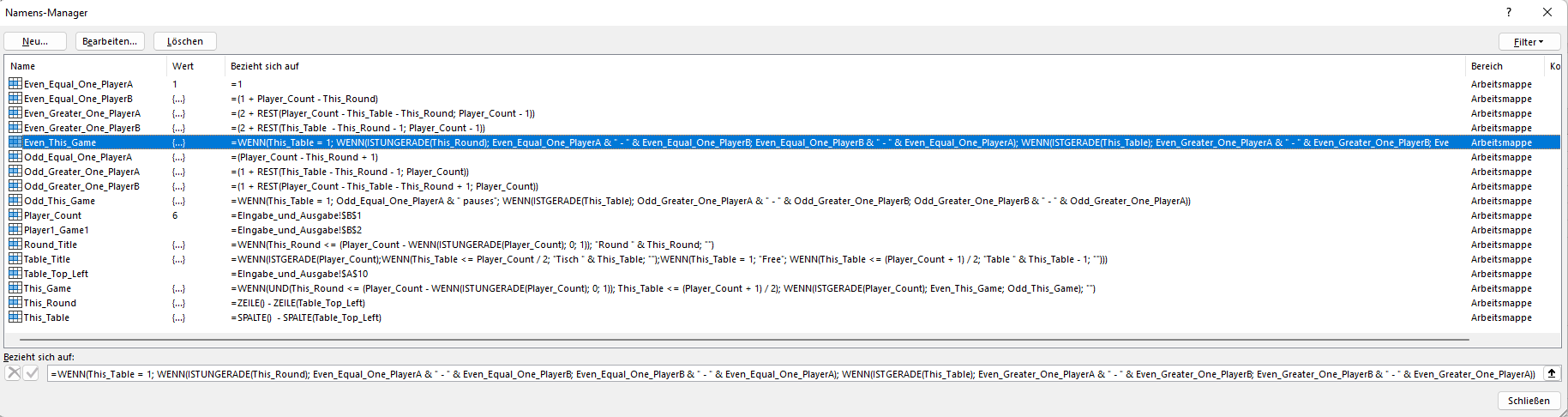
| Even_Equal_One_PlayerA | =1 |
| Even_Equal_One_PlayerB | =(1 + Player_Count - This_Round) |
| Even_Greater_One_PlayerA | =(2 + MOD(Player_Count - This_Table - This_Round, Player_Count - 1)) |
| Even_Greater_One_PlayerB | =(2 + MOD(This_Table - This_Round - 1, Player_Count - 1)) |
| Even_This_Game | =IF(This_Table = 1, IF(ISODD(This_Round), Even_Equal_One_PlayerA & " - " & Even_Equal_One_PlayerB, Even_Equal_One_PlayerB & " - " & Even_Equal_One_PlayerA), IF(ISEVEN(This_Table), Even_Greater_One_PlayerA & " - " & Even_Greater_One_PlayerB, Even_Greater_One_PlayerB & " - " & Even_Greater_One_PlayerA)) |
Example for an Odd Number of Players
| Free | Table 1 | Table 2 | Table 3 | |
|---|---|---|---|---|
| Round 1 | 7 pauses | 1 - 6 | 5 - 2 | 3 - 4 |
| Round 2 | 6 pauses | 7 - 5 | 4 - 1 | 2 - 3 |
| Round 3 | 5 pauses | 6 - 4 | 3 - 7 | 1 - 2 |
| Round 4 | 4 pauses | 5 - 3 | 2 - 6 | 7 - 1 |
| Round 5 | 3 pauses | 4 - 2 | 1 - 5 | 6 - 7 |
| Round 6 | 2 pauses | 3 - 1 | 7 - 4 | 5 - 6 |
| Round 7 | 1 pauses | 2 - 7 | 6 - 3 | 4 - 5 |
To create pairings for an odd number of players we do: In round 1 the last player pauses, in the second round the last but one does not play, etc. In round 1 player 1 plays against the last but one player, the second players starts against the antepenultimate player, etc., with alternating colours. In the following rounds at tables greater 1 each player will be substituted by the player with the next lower player number (the formula shows the summand - This_Round again), and player 1 will be substituted by the last one.
Then the following names are:
| Name | Refers to |
|---|---|
| Odd_Equal_One_PlayerA | =(Player_Count - This_Round + 1) |
| Odd_Greater_One_PlayerA | =(1 + MOD(This_Table - This_Round - 1, Player_Count)) |
| Odd_Greater_One_PlayerB | =(1 + MOD(Player_Count - This_Table - This_Round + 1, Player_Count)) |
| Odd_This_Game | =IF(This_Table = 1, Odd_Equal_One_PlayerA & " pauses”, IF(ISEVEN(This_Table), Odd_Greater_One_PlayerA & " - " & Odd_Greater_One_PlayerB, Odd_Greater_One_PlayerB & " - " & Odd_Greater_One_PlayerA)) |
A small quiz question: Why does the name Odd_Equal_One_PlayerB does not exist?
Answer: Because the formulas treat the pausing player as table 1, and in case of an odd number of players the table numbers are artificially reduced by 1 - please refer to the formula Table_Title.
Another small quiz question: How can you extend this solution to calculate the pairings for several tournaments in one Excel file?
Answer: Create all named ranges as local names in the current tab. Then copy this tab as often as necessary. Unfortunately you cannot just define the named ranges Player_Count and Table_Top_Left locally. All named ranges need to exist as often as the number of tournaments you want to calculate.
Appendix – Solution with Excel Worksheet Functions
An interesting fact: You can use this approach for (almost) any number of players. Just copy the rows down as far as necessary and the columns to the right until you see empty cells.
These formulas even work for pathological cases of 0 players, 1 player, and 2 players.
Download
Please read my Disclaimer.
sbRoundRobin.xlsx [20 KB Excel file, open and use at your own risk]
Note: A more general solution for round robin tournaments you can find under sbRoundRobin. You can choose the colour of the first game for player 1 and an additional output matrix will be created.